Machine learning

Support vector machine is a powerful tool, and we believe that every data scientist needs to know the internals of this machine learning algorithm. We are going to discuss the idea behind this classification algorithm in the proceeding paragraphs.

Given a hyperplane wx+b=0 we can define two additional hyperplanes that are parallel to and equidistant from the given one. Namely, wx+b=1 and wx+b=-1. If we say that we have a set of points $$(x_i, y_i)$$ where $$y_i$$ is either one or negative one (depending on the class to which the sample belongs), we state that the following must hold $$y_i(wx+b)-1 \geq 0$$, with equality occurring when points are exactly on the hyperplanes. We visualize the problem for the 2-D setting in the figure below:

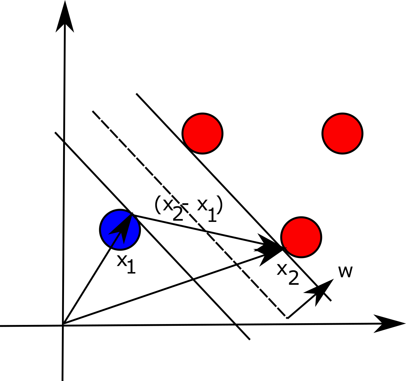
Now if we take two datapoints, one on each hyperplane, parallel to and equidistant to wx+b=0, $$x_1$$ and $$x_2$$, the margin between these two points can be expressed as follows (basically, the difference between the two vectors projected onto unit vector w, which is perpendicular to hyperplane that separates the points in different classes):

$$\frac{(x_2-x_1)\cdot w}{||w||}=\ \frac{2}{||w||}$$

According to SVM, the goal is to maximize this distance to reduce the classification error. However, maximizing this expression is the same as minimizing the following:

$$\frac{1}{2}{||w||}^2$$

Since we are given constraints in a form yi(wx+b)-1≥0 we can use Lagrange multipliers and construct the following equation:

$$L=\frac{1}{2}w^Tw-\sum_{i=1}^{n}{\alpha_i (y_i (wx_i+b)-1)}$$

To minimize this function, we need to find the partial derivatives with respect to vector w and b:

$$\frac{\partial L}{\partial w}=w-\sum_{i=1}^{n}{\alpha_iy_ix_i}\ =\ 0$$

$$\frac{\partial L}{\partial b}=\sum_{i=1}^{n}{\alpha_iy_i}=0$$

If we now plug in the values for w into the original equation and reduce it (here we also use the result for the second partial derivative), we obtain (dual optimization problem):

$$L_D=\sum_{i=1}^{n}\alpha_i-\frac{1}{2}\sum_{i=1}^{n}\sum_{j=1}^{n}{\alpha_i\alpha_jy_iy_jx_ix_j}$$

$$s.t. \sum_{i=1}^{n}{\alpha_iy_i=0}$$

We can now solve this maximization problem using Quadratic Programming (QP) solver and obtain Lagrange multipliers. Once this is done, we can find the vector w and bias term b. For the last point, we can take a point $$(x_s, y_s)$$ on the hyperplane:

$$y_s(wx_s + b)=1\ \rightarrow\ b=\ y_s-wx_s=y_s-\sum_{i=1}^{n}{\alpha_iy_ix_i}x_s$$

The derivations that we have presented are good only for linearly separable samples, however, one can use so called kernel trick to classify more complex datasets.